Transfer Learning for Multi-Class Scene Classification
Fine-tuned pre-trained models (ResNet, EfficientNet, VGG) for 6-class scene recognition with data augmentation in TensorFlow/Keras.
Overview
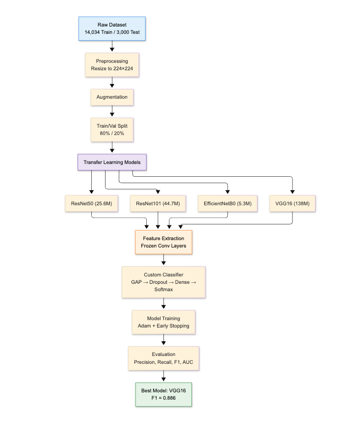
This project applies transfer learning to classify images into 6 scene categories (buildings, forest, glacier, mountain, sea, street) using pre-trained models like ResNet50/101, EfficientNetB0, and VGG16 on a dataset of ~14,000 images.
Implemented in TensorFlow/Keras, it incorporates data augmentation, early stopping, and multi-class metrics, with VGG16 achieving the highest F1-score of 0.886. The work demonstrates efficient handling of small datasets through feature extraction and fine-tuning.
Dataset
The Intel Image Classification dataset contains ~17,000 RGB images (150x150 pixels) across 6 natural scene classes,
sourced from various global locations. Split into training (14,034 images) and test (3,000 images) sets, with class
distribution as follows: buildings (2,627), forest (2,745), glacier (2,957), mountain (3,037), sea (2,784), street (
2,883). Images were resized to 224x224 and augmented for robustness.
For more details, refer
to dataset documentation.
Core Challenge: Managing class imbalance and varying scene complexities through transfer learning and augmentation.
Methodology

The pipeline starts with data preprocessing and augmentation, followed by model creation using frozen pre-trained bases, and ends with training/evaluation.
Stage 1: Data Preprocessing and Augmentation
Images are augmented to improve robustness:
train_datagen = ImageDataGenerator(
    rescale=1.0 / 255,
    rotation_range=20,
    width_shift_range=0.2,
    height_shift_range=0.2,
    shear_range=0.2,
    zoom_range=0.2,
    horizontal_flip=True,
    fill_mode="nearest",
    validation_split=0.2
)

train_generator = train_datagen.flow_from_directory(
    "data/seg_train",
    target_size=(224, 224),
    batch_size=32,
    class_mode="categorical",
    subset="training"
)
- Validation uses 20% split; test generator is unaugmented for fair evaluation.
Stage 2: Model Creation with Transfer Learning
Pre-trained models are adapted by freezing base layers and adding custom heads:
def create_model(base_model_class, learning_rate=1e-4):
    base_model = base_model_class(weights="imagenet", include_top=False, input_shape=(224, 224, 3))
    for layer in base_model.layers:
        layer.trainable = False
    model = Sequential([
        base_model,
        GlobalAveragePooling2D(),
        BatchNormalization(),
        Dropout(0.2),
        Dense(256, activation="relu", kernel_regularizer=l2(0.001)),
        Dense(6, activation="softmax")
    ])

    model.compile(
        optimizer=Adam(learning_rate=learning_rate),
        loss="categorical_crossentropy",
        metrics=["accuracy"]
    )
    return model
Stage 3: Training and Evaluation
Models train for 50 epochs with callbacks:
def get_callbacks(model_name):
    return [
        ReduceLROnPlateau(monitor='val_loss', factor=0.3, patience=5, min_lr=1e-6),
        EarlyStopping(monitor='val_loss', patience=7, restore_best_weights=True),
        ModelCheckpoint(filepath=f"{model_name}_best_model.keras", monitor='val_loss', save_best_only=True)
    ]

    history = model.fit(
        train_generator,
        validation_data=validation_generator,
        epochs=50,
        callbacks=get_callbacks(model_name)
    )
- Evaluation computes precision, recall, F1, AUC on test set.
-
Results

| Model | Precision | Recall | F1 Score | AUC |
|---|---|---|---|---|
| ResNet50 | 0.7306 | 0.7280 | 0.7262 | 0.9441 |
| ResNet101V2 | 0.7003 | 0.6997 | 0.6979 | 0.9333 |
| EfficientNetB0 | 0.0494 | 0.1673 | 0.0761 | 0.7283 |
| VGG16 | 0.8863 | 0.8857 | 0.8856 | 0.9881** |
- VGG16 outperforms others, with steady convergence and minimal overfitting.
Key Insights
- VGG16 Superiority: Excels due to its depth for feature extraction, achieving 88.6% accuracy despite small data.
- EfficientNetB0 Struggles: Poor performance (16.7%) suggests it’s less suited for this dataset without full fine-tuning.
- Augmentation Impact: Helps mitigate imbalance, but class similarities (e.g., glacier/mountain) limit perfect scores.
Learnings
- Why transfer learning is effective for small datasets, leveraging pre-trained features?
- When to frozen layers vs. fine-tune entire models?
- How to handle class imbalance with augmentation and careful evaluation metrics?
All the above questions were answered through this project, and it was a great learning experience.
This project highlights efficient use of transfer learning for practical image classification, with clear potential for extension to larger datasets.